


Top 4 Pocket WiFi and Portable Hotspot Router for Japan 2023
4 Best Pocket WiFi and Portable Hotspot Router for Japan in 2023 Planning a trip to Japan? Want to stay connected while exploring the beautiful …
Read Article
Google Sheets is a free online application that provides extensive spreadsheet features. One of the important features is the ability to wrap text in table cells. This is useful for creating more readable and organized documents.
In this article, we will look at two simple methods to wrap text in Google Sheets cells. Both methods do not require special programming skills or the use of special formulas.
The first method is to use the “Transfer by Word” option. This allows text to automatically move to the next line if it doesn’t fit in the current cell. Simply select the cell or range of cells where you want to wrap the text and right-click. In the context menu that appears, select “Transfer by word”. The text will now be more easily readable.
The second method is to change the line height. If you prefer to see all the text on one line, you can change the line height to make the text fit. Select the cell or range of cells where the text is located and choose the “Format” menu. Then select “Row Height” and set it to the desired value. The text will automatically wrap horizontally according to the specified line height.
Google Sheets are online spreadsheets that allow users to create, edit and store data. One of the useful features in Google Sheets is the ability to wrap text, which helps to improve the appearance of the table and make it more readable.
There are two easy ways to wrap text in Google Sheets:
Теперь текст будет автоматически обернут в ячейках, и ширина каждой ячейки будет подгоняться соответствующим образом, чтобы вместить весь текст.
Если вы хотите самостоятельно задать места переноса текста, вы можете использовать символ переноса строки.
Пример:
| Исходный текст: | Этотекстс переносами строки. |
| Обернутый текст: | Этотекстс переносами строки. |
Таким образом, можно обернуть текст в Google Sheets, используя автоматическую подгонку ширины ячейки или символ переноса строки. Оба способа позволяют изменить внешний вид таблицы и сделать ее более удобной для чтения.
Работа с таблицами является неотъемлемой частью многих проектов и задач. Google Sheets provides powerful table tools that can make your work much easier and faster.
Below are two simple methods to help you work successfully with tables in Google Sheets.
When text is in a table cell and you want it to appear in multiple rows in that cell, you can use the “Wrap Text” feature. This is especially useful when the text is long or when you want to add line breaks.
To wrap text in Google Sheets, select the cells where you want to wrap text. Then go to the Format menu and select Text Alignment. In the window that opens, check the box next to the “Transfer Text” option and click “Done”. Now the text will be displayed in multiple rows in the selected cells.
Often you want to add automatic row or paragraph numbering before the text in a table. In Google Sheets, you can easily add automatic numbering using the Counter and Control Number functions.
To add automatic row numbering, highlight the column where you want to add numbers. Then enter the formula =COUNT($A$1:A1) in the first cell of the column and copy it down the entire column. Now each cell in the selected column will contain the current row number.
To add automatic item numbering, use the Control Number feature. Highlight the column in which you want to add item numbers. Then enter the formula =CONTROLL!$A1 in the first cell of the column and copy it down the entire column. Now each cell in the selected column will contain the item number.
Read Also: Google Pixel 2 Screen Black and Won't Turn On: Troubleshooting Guide
Now you know two simple methods that will help you work successfully with tables in Google Sheets. Apply them in your projects and tasks to work more conveniently and efficiently.
In Google Sheets, there are several ways to wrap text in table cells. Discussed below are two simple methods that will help you accomplish this task successfully.
Navigate to the cell you want to wrap and right-click. From the context menu, select “Change Column Widths/Auto Adjust”. The text will be wrapped to fit in the cell. 2. Method 2: Using the line break character
Navigate to the cell where the text is to be wrapped. Then click on the desired location where you want to do a line break and type the line break character by pressing the “Enter” or “Return” key. The text will wrap on the next line within the cell.
Choose the most convenient method for you to wrap text in Google Sheets and continue to successfully work with the data in your spreadsheet!
One way to wrap text in Google Sheets is to use the built-in “Wrap Text” feature. By following a few simple steps, you can quickly and easily apply this feature to cells with your text.
Read Also: Devil may cry 6: what's next for the devils? Information about the new part of the popular game series
If you want to apply the Wrap Text feature only to specific cells in a column or row, you can select those cells before performing step 2. In this case, only the selected cells will be wrapped.
Method 1 is simple and effective for quickly wrapping text in Google Sheets cells. Now you know how to use the Wrap Text feature and enjoy the convenience of formatting your data.
The second method to wrap text in Google Sheets is to use cell formatting.
First, select the cell or range of cells where you want to wrap text. Then, go to the Format menu and select “Erase Cell Formatting.” This will remove any previous formatting settings.
Now, with the cell or range of cells selected, right click and select “Format Cell”. In the window that appears, click on the “Alignment” tab.
In the “General” section, you will find the “Word Reposition” option. Check the box next to this option to wrap the text in the cell by word.
You can also choose other options to move text around, such as “Transfer by Character”.
Once you have set the desired options, click the “OK” button to apply the formatting.
Now the text in the selected cell or range of cells will be wrapped by words or characters, depending on the selected settings.
So, using cell formatting is the second easy way to wrap text in Google Sheets and make it more readable.
To wrap text in a cell in Google Sheets, you need to select the desired cells, then right-click and select “Wrap Text”.
Yes, in addition to using the context menu, you can also wrap text by selecting the “Wrap Text” option from the “Format” menu in the top toolbar. You can also use the keyboard shortcut Ctrl + Shift + B.
There are two types of text wrapping available in Google Sheets: “Normal” and “Vertical”. Vertical wrapping allows you to place text vertically in a cell.
Yes, you can apply text wrapping only to specific cells. To do this, you need to select the desired cells and choose the “Wrap Text” option from the context menu or keyboard shortcut.
No, you cannot wrap text in a cell in Google Sheets using a formula. You can only perform this action using the context menu or keyboard shortcut.
There are two simple methods to wrap text in Google Sheets. The first method is to use the cell formatting. Highlight the text you want, right click and select “Format Cell”. Then in the “Alignment” section, select the desired text wrapping option. The second method is to use the Wrap function. Type the formula “=Wrap(text)” in the cell and press Enter. The text will be wrapped in the cell.
4 Best Pocket WiFi and Portable Hotspot Router for Japan in 2023 Planning a trip to Japan? Want to stay connected while exploring the beautiful …
Read Article
How To Fix Nintendo Switch Controller Won’t Turn On | New in 2023 Are you experiencing issues with your Nintendo Switch controller not turning on? …
Read Article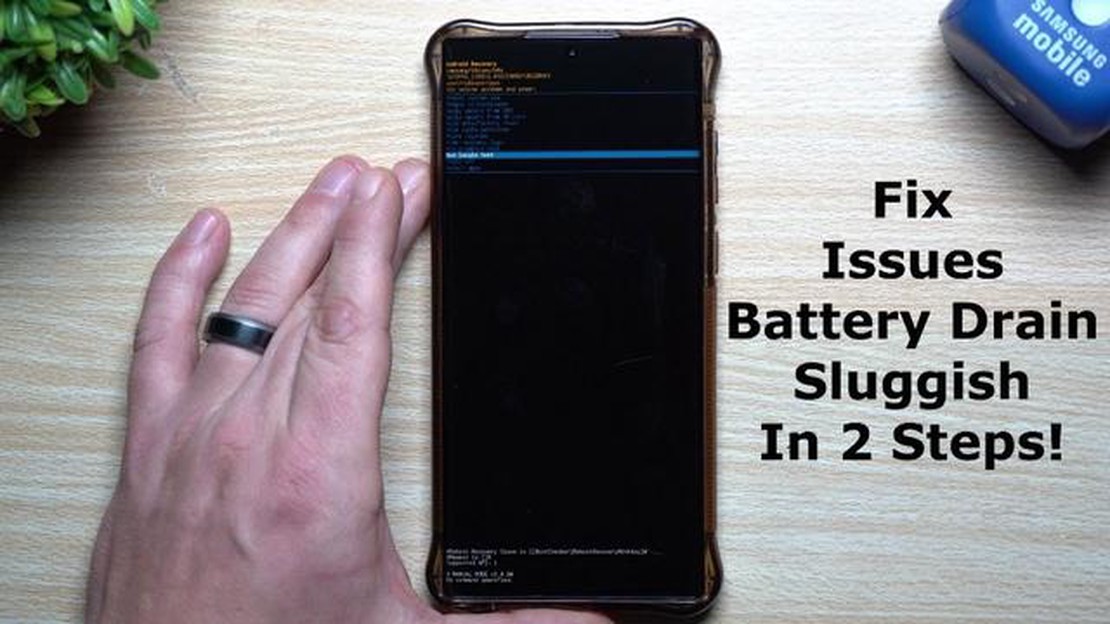
How to fix your Samsung Galaxy A6 2019 battery that drains so quickly after an installing update (Troubleshooting Guide) The Samsung Galaxy A6 2019 is …
Read Article
Shadowy chrome extension steals $16,000 worth of cryptocurrency In recent years, cryptocurrencies have become one of the most popular targets of …
Read Article
Top 10 cmd commands useful in hacking No matter what role you play in the board game “Hacker”, mastery of command line commands (cmd) can be useful in …
Read Article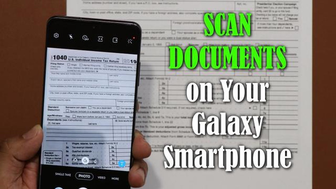
How To Scan Documents On Your Samsung Phone With the advancement of technology, scanning documents has become easier than ever. Gone are the days when …
Read Article


