Learn How To Multiply In Excel: A Step-by-Step Guide

How To Multiply In Excel

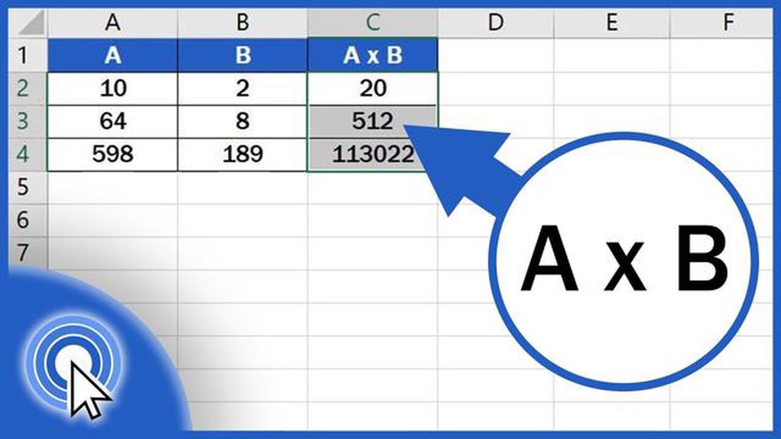
Excel is a powerful tool that allows you to perform complex calculations and operations with ease. One of the basic functions that you need to know is how to multiply in Excel. Multiplication is an essential operation when working with numerical data, and understanding how to use the multiplication formula in Excel is crucial for any user.

Table Of Contents

In this step-by-step guide, we will take you through the process of multiplying numbers in Excel. Whether you are a beginner or have some experience with Excel, this guide will help you master the multiplication function and apply it to your data.

To multiply in Excel, you need to use a simple formula. The formula for multiplication in Excel is =A1B1, where A1 and B1 are the cells containing the numbers you want to multiply. You can also multiply multiple cells by separating them with a comma. For example, =A1B1,C1*D1 will multiply the numbers in cells A1 and B1, and C1 and D1 respectively.

Tip: If you want to multiply a number by a constant, you can simply enter the constant in the formula. For example, =A1*5 will multiply the number in cell A1 by 5.

Once you have entered the formula, Excel will automatically calculate the multiplication and give you the result. The result will be displayed in the cell where the formula is entered. You can also format the cell to display the result in a specific format, such as currency or percentage.

Now that you know the basics of multiplying in Excel, you can apply this knowledge to your own data and calculations. Whether you are working on a budget, analyzing sales data, or performing any other calculations, the ability to multiply in Excel will make your work more efficient and accurate.

Understanding the Basics

Before diving into the process of multiplying in Excel, it’s important to grasp some fundamental concepts. Excel is a powerful spreadsheet software that allows you to perform various mathematical operations, including multiplication, with ease.

Here are a few key terms you should be familiar with:

Cell: In Excel, a cell is a small rectangular box where you can enter data or formulas. Each cell is identified by a unique combination of a column letter and a row number. For example, cell A1 is in the first column and first row.
Formula: A formula is an equation that performs a mathematical calculation. In Excel, formulas always begin with an equal sign (=). For multiplication, you’ll use the asterisk (*) symbol.
Range: A range refers to a group of cells. It can be a single cell, a row, a column, or a combination of multiple cells. Ranges are often used to apply formulas to multiple cells simultaneously.

Now that you understand these basic concepts, let’s explore how to multiply in Excel using different methods.

There are three main ways to multiply in Excel:

Using the formula bar
Using the multiplication operator (*)
Using the PRODUCT function

In the following sections, we will go through each of these methods in detail and explain how to apply them to your data.

Step 1: Select the Cells

The first step in learning how to multiply in Excel is selecting the cells you want to work with. Excel allows you to multiply values in multiple cells at once, but you need to specify which cells you want to include in the calculation.

To select the cells, you can click and drag your mouse over the desired range of cells, or you can use the keyboard shortcuts. Here are a few ways to select cells:

Click and drag: Click on the first cell you want to include in the multiplication, hold down the mouse button, and drag the cursor to select the remaining cells.
Shift key: Click on the first cell in the range, hold down the Shift key, and then click on the last cell to select all the cells in between.
Ctrl key: Hold down the Ctrl key and click on each individual cell you want to include in the calculation.

Once you have selected the cells, they will be outlined in a highlighted border. This indicates that the cells are now part of the current selection.

Read Also: How to Block A Number on Redmi Note 8 - Step-by-Step Guide

If you accidentally select the wrong cells or want to change your selection, you can simply click and drag your mouse over the correct range of cells, or use the keyboard shortcuts mentioned above.

Step 2: Enter the Formula

Select the cell where you want the result of the multiplication to appear.
Type the equals sign (=) to start entering a formula.
Enter the first number or cell reference that you want to multiply.
Type the asterisk (*) symbol, which represents the multiplication operation.
Enter the second number or cell reference that you want to multiply.
Press Enter or Return to complete the formula.

For example, let’s say you want to multiply the numbers in cell A1 and B1 and display the result in cell C1. Here’s how you would enter the formula:

A	B	C
5	10	=A1*B1

After you press Enter or Return, Excel will calculate the result of the multiplication and display it in the selected cell (C1 in this example).

You can also use cell references in the formula, allowing you to multiply different numbers in different cells without changing the formula. For example, if you want to multiply the numbers in cells A1 and B2 and display the result in cell C3, you would enter the formula =A1*B2 in cell C3.

Now that you know how to enter the formula, let’s move on to the next step to learn how to copy the formula to other cells.

Read Also: Apple's COVID-19 patient tracking service: defeat or victory?

Step 3: Apply the Formula to Multiple Cells

Now that we have learned how to multiply in Excel and have created a formula, we can apply it to multiple cells. This is particularly useful when working with large sets of data or when you need to perform the same calculation on multiple cells.

To apply the formula to multiple cells, follow these steps:

Select the cell that contains the formula you want to apply.
Click and hold the small square in the bottom-right corner of the selected cell.
Drag the square to the cells where you want to apply the formula.

Alternatively, you can also use the copy and paste method to apply the formula to multiple cells:

Select the cell that contains the formula you want to apply.
Press Ctrl+C to copy the formula.
Select the range of cells where you want to apply the formula.
Right-click on the selected range and choose “Paste” from the context menu.

By applying the formula to multiple cells, Excel will automatically adjust the cell references in the formula to match the new location. This means that if your original formula multiplies cell A1 by cell B1, when you apply the formula to cell C2, Excel will automatically update the formula to multiply cell C2 by cell D2.

Now that you know how to apply a formula to multiple cells, you can easily perform the same calculation on multiple data points and save time when working with large sets of data.

FAQ:

How do I multiply numbers in Excel?

To multiply numbers in Excel, you can use the multiplication operator () or the PRODUCT function. If you want to multiply two specific numbers, you can simply enter them in separate cells and use the multiplication operator between them. For example, to multiply 3 and 4, you can enter “=34” in a cell and press Enter. If you want to multiply a range of numbers, you can use the PRODUCT function. For example, if you have a range of numbers in cells A1 to A5, you can enter “=PRODUCT(A1:A5)” in a cell and press Enter.

Can I multiply numbers in Excel without using formulas?

No, you cannot multiply numbers in Excel without using formulas. Excel is a spreadsheet program that is designed to perform calculations using formulas. If you want to multiply numbers in Excel, you need to use either the multiplication operator (*) or a multiplication function like PRODUCT.

Can I multiply numbers and text in Excel?

No, you cannot multiply numbers and text in Excel. Excel is a numerical-based program, and it does not support multiplying numbers and text together. If you try to multiply a number and a text value, Excel will return an error.

What should I do if I get an error when trying to multiply numbers in Excel?

If you get an error when trying to multiply numbers in Excel, you should check your formula for any mistakes. Make sure you are using the correct syntax and that all the referenced cells contain valid numbers. If you are using a function like PRODUCT, make sure you are giving it the correct range of cells to multiply. If you are still having trouble, you can try using the Help feature in Excel or search for a solution online.

Can I multiply numbers in Excel and display the result as a fraction?

Yes, you can multiply numbers in Excel and display the result as a fraction. To do this, you can use the MIXED function or format the cell as a fraction. The MIXED function allows you to display a number as a mixed fraction, while formatting the cell as a fraction allows you to display the number as a simple fraction. Keep in mind that when you multiply numbers in Excel, the default format is a decimal, so you will need to change the format of the cell to display the result as a fraction.

How do I multiply two cells in Excel?

To multiply two cells in Excel, you need to enter the formula =cell1*cell2. Replace “cell1” and “cell2” with the actual cell references you want to multiply. Press Enter, and the result of the multiplication will appear in the cell where you entered the formula.

Can I multiply multiple cells in Excel?

Yes, you can multiply multiple cells in Excel by using the SUMPRODUCT function. The SUMPRODUCT function multiplies corresponding values in the specified arrays or ranges and returns the sum of those products. To use it, enter the formula =SUMPRODUCT(array1, array2, …) where “array1”, “array2” are the ranges or arrays you want to multiply. Press Enter, and the result will be calculated.