How to change the color of cell grid lines in Excel: a detailed guide

How to change the color of cell grid lines in excel?

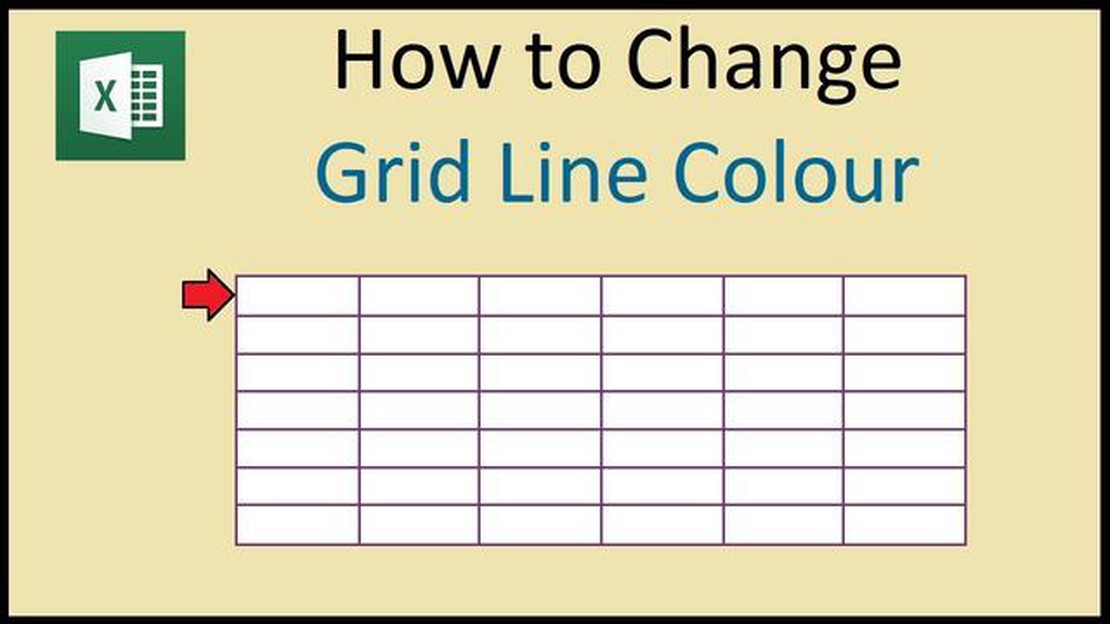
Excel is one of the most popular spreadsheet programs. One of the features of Excel is the ability to change the appearance of cells, including the color of the grid lines. This option can be useful when creating professional looking spreadsheets or when highlighting certain cells.

To change the color of cell grid lines in Excel, you will need to find the Design tab in the Excel menu. On this tab, you will be able to choose the color of the grid lines or apply specific styles to the cells. If you only want to change the color of the grid lines, you can select the “Line Color” option and choose the desired color from the palette.

Table Of Contents

If you need to change the color of the grid lines of only specific cells, you need to select those cells with the mouse cursor. You can then apply the changes only to the selected cells using the same tools on the Design tab.

Changing the color of cell grid lines in Excel can be useful when creating professional reports or charts. When you learn how to use this feature, you can create more attractive and readable Excel spreadsheets.

How to change the color of cell grid lines in Excel: a detailed guide

In Excel, you can change the color of cell grid lines to make your spreadsheet more aesthetically pleasing or to highlight certain data. This guide will present the steps to change the color of cell grid lines in Excel.

Launch Excel and open the document in which you want to change the grid color.
Highlight the cells for which you want to change the grid color.
On the top toolbar, find the Borders tab and click it.
From the menu that opens, select the Cell Rulers option.
In the window that appears, select the “Color” tab and select the desired cell grid color.
After selecting the color, the cell grid will automatically change.
Click on the “OK” button to confirm the changes.

In this way, you can easily change the color of cell grid lines in Excel. This is a simple and effective feature that allows you to customize the appearance of your spreadsheet and highlight important data.

Options to change the grid color in Excel

When you work with spreadsheets in Excel, the cell grid can make your work more convenient and systematized. The default cell grid color is called “Automatic” and can be changed in several ways. In this article, let’s look at the main ways to change the grid color in Excel.

1- Changing the grid color for the whole sheet:

Right-click on the sheet tab at the bottom of Excel.
Select “Change tab color” from the context menu.
Select the desired grid color.

Change the grid color for specific cells:
Highlight the cells for which you want to change the grid color.
Right-click and select “Format Cells” from the context menu.
Click the Fill tab.
Select the desired grid color.
Click “OK” to save the changes.

Read Also: How To Fix “Windows Cannot Complete The Extraction” Error (Updated 2023) - [Your Website Name]

7. Change the grid color for the entire table:

8. Highlight the entire table for which you want to change the grid color. 9. Right-click and select “Table Format” from the context menu. 10. Click on the “Grid and Lines” tab. 11. Select the desired grid color and line thickness. 12. Click “OK” to save the changes.

Changing the grid color in Excel can help make your spreadsheet more visually appealing and easier to read. You can experiment with different color options to find the best fit for your project.

Read Also: Download and install Windows 11 now: process and detailed instructions

Table: Steps to change the grid color in Excel

No. of step	Options for changing the grid color
1	Changing the grid color for the whole sheet
2	Change the grid color for specific cells
	3

Changing the grid color for cells in Excel: step-by-step instructions

Excel is one of the most popular programs for working with tabular data, and the ability to customize the appearance of a table makes it much easier to understand information. One of the main aspects of a spreadsheet’s appearance is the color of the cell grid. In this step-by-step instruction, you will learn how to change the color of cell grid lines in Excel.

**Open Excel and select the table you want.**If you have already created a table, open it in Excel. If not, create a new table.
Select the cells whose grid color you want to change. To select multiple cells, hold down the Ctrl key on your keyboard and click on the desired cells.
Open the Borders menu of the Home tab. The Home tab is at the top of the screen, at the top of Excel. The “Borders” menu has several different options for customizing the cell grid.
Select the Border Color option. This option allows you to customize the color of the cell grid lines. After selecting the option, the color palette will open.
**Select the desired color from the palette.**Click the desired color in the palette to apply it to the selected cell grid.
**Check the changes.**When you have selected a color for the cell grid, you will see that the corresponding lines in the table have changed color.

Now you know how to change the color of cell grid lines in Excel. This feature allows you to customize the appearance of the table and make it more visually appealing. Experiment with different colors and create memorable tables in Excel!

FAQ:

Can I change the color of grid lines only in a certain part of the table?

Yes, you can change the color of grid lines only in a specific part of the table. To do this, you need to select the desired cells (or a range of cells) and apply the new gridline color to them using Excel’s formatting tools.

What other ways can I change the gridlines in Excel?

In addition to choosing the color of the grid lines, there are other ways to change the appearance of the grid lines in Excel. These include changing the thickness of the lines, adding and removing specific grid lines, and changing the style (dashed, solid, etc.). All of these settings can be customized in the cell formatting menu under “Borders”.

How do I change the color of cell grid lines in Excel?

To change the color of cell gridlines in Excel, you need to select the desired cell range, then go to the “Style” tab and click on the “Gridlines” button. A list of available colors will appear, where you can select the one you want. You can also customize the thickness of the lines, add or remove lines.